Advances in our understanding of the structure, composition, dynamics and evolution of the Earth's atmosphere have come about because of studies conducted by scientists and engineers from a broad range of disciplines, including, among others, meteorologists, spectroscopists, and physicists. Principles from physics, chemistry and mathematics are used in all aspects of atmospheric research. Since these are subjects that are also fundamental to the education of chemical engineers, many chemical engineers have chosen careers aimed at solving atmospheric problems. One focus has been on understanding of climate change, in part because of the strong link between climate change and the Earth's chemical composition. In this section we briefly describe the structure of the Earth's atmosphere, how some simple chemical engineering principles are used to detect and describe changes in the atmospheric chemical composition, and how pollutants are believed to affect the Earth's climate.

The figure below shows a schematic of the Earth's atmosphere that includes a sketch of the variation in air temperature with height. The lowest layer of the atmosphere, in which we live, is called the troposphere. Temperature decreases with height in the troposphere, as anyone who has flown on an airplane will have noted. The troposphere is also the layer in which "weather" is experienced: clouds, rain and snow precipitation, hurricanes and tornadoes, and thunderheads and lightning are all observed in the troposphere. You may have observed the formation of a thundercloud and noted that the very high top of the cloud "flattened out", or appeared to "bubble over". This happens when the cloud motions are so vigorous that the cloud grows through the depth of the troposphere and hits the barrier known as the tropopause. At the tropopause, the dependence of air temperature with height is reversed: temperature begins to increase with altitude. This type of temperature profile is called a stable profile, because rising air parcels lose bouyancy - the air surrounding them is warmer than they are, and they tend to sink instead of rise. (Think about what happens if you add cold cream to a cup of hot coffee.) The tropopause thus acts like a "lid" for the troposphere and prevents mixing of air across it into the next layer, the stratosphere.

The layers in the atmosphere can be identified by the strong variations in the temperature profile.

The stratosphere is characterized by an increasing temperature profile with height, called an "inversion", and very stable, turbulence-free air. The stratosphere is also very dry because moisture that is evaporated from the Earth's surface from oceans and land cannot rise past the lid presented by the tropopause. As shown in the figure, commercial and supersonic aircraft fly in the tropopause / lower stratosphere regions—above the "weather"— because of the reduced drag from the thin air and the low turbulence. The cause of the stratospheric temperature inversion is the stratospheric ozone layer, concentrated near 25 km altitude. Ozone (O3) absorbs ultraviolet solar radiation, in turn raising the temperature. Although ozone that forms near the surface of the Earth in polluted regions is considered harmful to human health, the stratospheric ozone layer is extremely beneficial: it helps maintain the troposphere / stratosphere temperature inversion, and it absorbs solar ultraviolet radiation before it can reach the surface and cause damage to biological organisms, including skin cancer in humans.

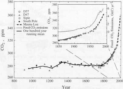
Two of the simplest, yet most useful, engineering principles that are applied to the atmosphere are the concepts of mass and energy balances. To illustrate the first type of balance, imagine a leaky bucket—one with a hole near its bottom. If the bucket is initially filled with water, the water level drops as water leaks out of the bucket. Water could be supplied to the bucket by placing it under a tap and turning on the faucet. If the flow rate from the faucet is adjusted to exactly match the leak rate, the water level remains constant. If the faucet supplies water at a slower or faster rate, then the water level continuously drops or rises, and the rate of change of the water level depends upon how different the supply and loss rates are. Although this example is extremely simple, it illustrates the basic idea behind constructing budgets for different chemical components in the atmosphere. We need to measure the rate at which the component enters the atmosphere (emission rate), the rate at which it leaves the atmosphere (sink rate), and its current level (atmospheric concentration) along with the rate of change of that level, which can be zero if the budget is "balanced" — i.e., if the emission rate equals the sink rate. Let's examine the global budget of carbon dioxide, CO2, as a relevant example. Carbon dioxide is taken up from the atmosphere by plants during their growth cycle, when they convert CO2 and water into oxygen and biomass. Some carbon dioxide can also be dissolved into the world's oceans, although this is a rather slow process. These two processes are the major sinks for atmospheric CO2. The sources of CO2 include the decay of dead plants, natural combustion processes (e.g., burning of forests by wildfires), and combustion processes due to human activity, which include gasoline burning, coal burning to produce power, and burning to clear land for agricultural activities. The natural emissions and sinks are ten times larger than the source due to human activity, and are approximately in balance. The figure below shows the atmospheric concentration of CO2 from about the year 1000 A.D. to the present. (The early data are obtained from ice cores that are drilled from polar regions. Bubbles of air trapped in the ice at various depths are then analyzed for atmospheric chemical composition during the era represented by that ice section.) The notable feature in the timeline is the sharp increase in atmospheric CO2 concentrations after about the mid-1800's. Prior to this time, the global cycle must have been approximately in balance, since atmospheric concentrations did not change significantly. The timing of the sudden increase coincides with the start of the Industrial Revolution, when for the first time in history large amounts of fossil fuels (coal, oil and natural gas) were burned for powering engines and producing electricity. The result was that the number of sources of CO2 to the atmosphere was abruptly increased, throwing the budget out of balance and, over time, causing a dramatic increase in atmospheric concentrations of CO2; the sources exceeded the sinks.

Atmospheric CO2 concentrations over the past 1000 years from the recent ice core record and (since 1958) from a measurement site on the Mauna Loa volcano. The solid curve is based on a 100 running average.

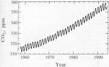
A more detailed look at changes in CO2 is given in the following figure, which shows data from Mauna Loa in Hawaii from the late 1950's to the present. There is a pronounced annual cycle in CO2 concentrations when viewed at a single site, rather than as a global average. At Mauna Loa, this is due to the annual cycle of growth and decay of plant life in land masses north of the equator; the air affected by these sources and sinks is sampled at the Mauna Loa site. If only those natural sources and sinks were present, the annual cycle would remain in the data, but the overall trend of the data would be flat — that is, the average would not increase over the decade from 1960 to the present. Instead, the small (~10%) annual perturbation in the budget that is due to fossil fuel burning in the Northern Hemisphere constitutes a net, unbalanced source that produces the observed upward trend with time.

The CO2 concentration in the atmosphere measured at Mauna Loa, Hawaii, since 1958, showing trends and seasonal cycles.

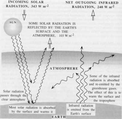
The figure below shows an accounting of what happens to the energy from the Sun that strikes the Earth. Because the Earth's overall energy budget is in balance, the energy leaving must equal the energy coming in (about 343 watts per square meter, or W m–2). However, the form of the energy does not necessarily have to be the same entering or leaving, and indeed it is not the same because of interactions with the atmosphere. The energy from the Sun is concentrated in the visible and ultraviolet part of the energy spectrum. Some of this light energy (about 103 W m–2) bounces back to space when it hits the atmosphere. The remainder hits the surface of the Earth and is absorbed. It is re-emitted, but now as thermal energy (longer-wavelength, or infrared, radiation) that eventually leaves the atmosphere to complete the energy budget. Before it leaves, however, it interacts with "greenhouse gases" in the atmosphere that can absorb and re-emit energy with these longer wavelengths (but that cannot interact with the shorter-wavelength solar energy). The absorption and re-emission have the effect of warming the surface and the troposphere, creating the warmer temperatures that support life as we know it.

A schematic of Earth's overall energy balance. The net input of solar radiation must be balanced by the net output of infrared radiation. About one-third of incoming solar radiation is reflected and the remainder is mostly absorbed by the surface.

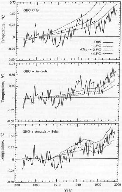
What factors could change this energy balance? Consider first changes in the amounts of greenhouse gases—a subject that has been the focus of intense international scientific and public interest. The most-discussed greenhouse gas is carbon dioxide (CO2), which is a product of any combustion process that burns carbon-containing fuels. These include grasslands, wood, peat, coal, and oil. Higher levels of CO2, created by increased global industrialization, increase the absorption of infrared radiation from the Earth's surface. However, the atmosphere must still radiate 240 W m–2 of thermal energy to space. To fulfill this requirement, the temperature rises, because emission of thermal energy increases with temperature. This brings the energy budget back into balance, but the net effect is that tropospheric temperatures are increased when CO2 levels rise. For a different scenario, consider next only the solar radiation that is immediately reflected back to space. Clouds and pollutants present in the atmosphere are responsible for some of this reflection. If global cloudiness changes, or if global pollution levels rise, then more than 103 W m–2 could be bounced back to space. Since the total energy in must still equal the total energy out, that leaves less solar radiation to penetrate to the surface, be re-emitted, and interact with greenhouse gases. The overall result would be a cooling of the surface and troposphere, relative to today's temperatures. Many scientists believe that some of this cooling has taken place, and has counteracted global warming from increases in greenhouse gases. The figure below, which shows observations of global temperature compared with model predictions, provides support for these ideas. In the top panel, the observations since the late 1800's, shown by the solid line, are compared against model predictions that include only the effects of rising global greenhouse gas concentrations. There is a range of model predictions because there is still much uncertainty in how to correctly simulate the many complex processes occurring in the atmosphere. Nevertheless, most of the models predict more warming than has been observed. In fact, such discrepancies between observations and models has led to much skepticism of their use in projecting climate change, and criticism of basing international policy decisions related to greenhouse gas emissions on such simulations.

A comparison of observed and modeled (predicted) global mean temperatures. The solid line in each plot represents the actual observed temperature, while the dashed lines indicate predicted values.

However, as can be seen from the middle and bottom panels in the figure, the modeling approach itself is not completely to blame: the model must be supplied with enough detail to mimic all the processes that are important. A fuller understanding of the various factors that can contribute to global warming or cooling has helped improve the agreement between observations and model predictions substantially. In the middle panel, the cooling effects due to rising levels of pollutants in the form of particles ("aerosols") has been added to the greenhouse gas effects. This counteracting cooling creates a modeled trend much closer to the global temperature trend. In the bottom panel, both effects are included along with simulated variations in the energy output of the Sun, which has its own multiyear cycle. The solar variations reproduce some of the fine structure in the observational trend. The enhanced understanding that has made such accurate simulations possible in recent years has come about because of contributions from scientists and engineers from many disciplines who have individually studied the various components of the global energy budget and suggested how these contribute to the overall "big picture".

In the above discussion, pollution in the form of atmospheric particles — also called "aerosols" — was implicated in changes in the global energy budget because of the particles' activity in reflecting incoming solar radiation back to space. Particles in the atmosphere can interact with light not only in this way, but also such that they affect visibility. This is shown in the accompanying figure. An observer perceives an object because light strikes that object and reflects into the eye of the observer. The reflected light carries information about the object, including its color. Particles in the atmosphere interfere with perception of the object in several ways. The light reflected from the object can be scattered out of the observer's line of sight, or absorbed before it reaches the observer; the intensity of the perceived image is thereby lessened. Sunlight can also be bounced into the observer's line of sight from the atmosphere around the object; this light carries no information about the object and thus just serves to obscure the image (a similar effect as glare from oncoming headlights that obscures vision of the road ahead). Visibility is measured in terms of visual range, the farthest distance that a dark object on the horizon can just be perceived. The higher the concentration of particles in the atmosphere, the shorter the visual range.

Contributions to atmospheric visibility include light from a target (e.g., the mountains) reaching the observer, light from the target scattered away from the observer's line of sight, and sunlight scattering into the observer's line of sight.

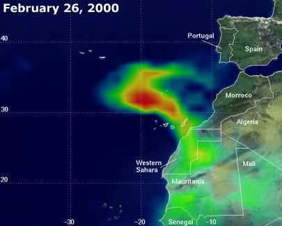
What are the sources of atmospheric particles? There are some very large, episodic sources that are natural in origin. The first figure below shows a satellite image of a dust storm in the Sahara that has lifted huge quantities of soil particles into the mid-troposphere. Such dust storms recur each year in Africa in the summertime, when meteorological patterns create intense convective (lifting) activity in the region and prevailing winds sweep the aerosols across the Atlantic Ocean. Saharan dust is detected annually in Bermuda, Barbados, and the southeastern U.S., and has been shown to be responsible for episodes of poor visibility in Florida. (Interestingly, the minerals in the dust that falls into the Atlantic Ocean during transit are important sources of nutrients to marine life.) There are also large sources of dust in Asia during the springtime, again when weather patterns favor lifting and transport eastward, out across the Pacific. Asian dust is frequently detected at Mauna Loa and occasionally along the West Coast of the U.S. The second figure shows just how far the Saharan dust can persist as it travels almost due west across the Atlantic towards Central and North America.

This February 26, 2000 image shows a dust plume obtained from TOMS (Total Ozone Mapping Spectrometer) data over the Sahara Desert and extending over the Atlantic Ocean and Canary Islands. The land sources of the dust plume are clearly visible, with the main source coming from Western Sahara and Mauritania. The green to red false colors in the dust plume image represent increasing amounts of aerosol, with the densest portion over the ocean. Under the densest portions of the dust plume (red) the amount of ultraviolet sunlight is reduced to half its normal value, while over the land (green) the UV sunlight is reduced by about 20%. The high dust amount over the ocean was not present on previous days. Between February 27 to February 29 the ocean dust plume decreases while a massive dust plume develops over the land that covers a region from the equator to 30o N latitude. Based on previous dust events observed by TOMS, there should be another dense plume over the ocean during the next few days.

A TOMS satellite image showing transport of aerosols (i.e., dust) from their source in Saharan Africa, on July 10, 1999.

Another large, episodic, natural source of particles is fires, usually initiated by lightning strikes during thunderstorms. In some years, drought conditions encourage frequent and fast-spreading fires that combust large numbers of acres of forest or grassland. In some developing countries, including in Central and South America and in southern Africa, annual burning is used to clear cropland for planting. The smoke particles released by fires create local and sometimes long-range pollution problems. The figure below shows a satellite image that has captured one such smoke event in May 1998. Severe drought in Central America earlier that year left the region susceptible to uncontrollable fires, which began burning in early Spring and intensified in May. During that time of the year, prevailing winds usually shift, bringing air from Mexico into the southern U.S. This shift is captured in the image: the fires are located in the Yucatan and southern Mexico, and produced the heavy plume blowing west into the Pacific. The shifting winds, however, rapidly carried a secondary plume northward into the U.S., where the smoke was detected as far north as Wisconsin. The May 1998 fires and accompanying smoke were so severe, and persisted for so long, that Texas issued a public health advisory for most of the month, warning people to limit the amount of time spent out of doors.

A TOMS satellite image showing smoke transport across Central and North America, on May 18, 1998. Fires located in the Yucatan produced a plume which was carried as far north as Wisconsin.